Linear Quadratic Gaussian Control

This post gives a gentle introduction to the control theory and linear quadratic Gaussian control.

Introduction

The subject of control theory is a dynamical system. Let $\mathbf{x} \in \R^n$ denotes the state of the system, then

where $f: \R^n \to \R^n$ is a function, describes the system. For example, a moving particle in a field may be described by its position and velocity, a 2-dimensional space, and the physics of the system determines $f$. In general, determining $f$ is a hard physics problem which will not be the focus of this post. We will consider only linear systems, for which $f$ is a linear function, or we can simply write the system of equations as

where $A \in \R^{k \times k}$ In reality, $f$ is almost never linear, so we linearize the system around the fixed points, i.e., where $f(\mathbf{x}) = 0$, so that we can approximate the system near the fixed points as a linear system with $A = \frac{Df}{D\mathbf{x}}$, the Jacobian.

To control the system, we assume that we have $k$ control “knobs” which affects the system linearly,

where $B \in R^{n\times k}, \mathbf{u} \in R^k$. Here $B$ is completely determined by the physics of the control knobs, and it is fixed once the system is manufactured.

For linear closed-loop feedback control, we assume $\mathbf{u} = K\mathbf{x}$, where $K \in \R^{n\times k}$ is the control law. Therefore, the system of equations becomes

The solution to this system of first-order ODE is

where $TDT^{-1} = A-BK$ is the spectral decomposition. The stability of the system is determined by the eigen-values of $D$.

Linear Quadratic Gaussian

Linear Quadratic Regularizer

Linear Quadratic Regularizer assumes a quadratic cost with the form

where $Q, R \in \R^{n \times n}$, and $\bar{\mathbf{x}}$ is the desired state.

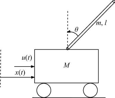Figure 1. Inverted Cart Pole Problem.

For example, consider a inverted cart pole problem, where the state space is $\mathbf{x} = (x, \dot{x}, \theta, \dot{\theta})$. Consider the desired state $\bar{\mathbf{x}} = (0,0,\pi,0)$, which is also a fixed point to linearize around. Assume there is no friction, then

We can define the cost matrices as

The Linear Quadratic Regularizer finds the optimal control law $K$ such that

is minimized as long as the system is controllable.

Kalman Filter

In reality, often we cannot measure the full state of the system. The Kalman Filter allows us to measure only a partial state, and recover an estimation of the full state together with the control input. Suppose the measured values are $\mathbf{y} = C \mathbf{x}$, where $C$ is a matrix and $\mathbf{y}$ is a smaller vector. The Kalman Filter defines the Kalman Filter solves for the optimla Kalman Filter gain $K_f$ to estimate the state $\mathbf{\hat{x}}$ from $\mathbf{y}$, such that the estimate is updated according the following ODE:

where $\hat{\mathbf{y}} = C \hat{\mathbf{x}}$. Intuitively, the Kalman Filter is a closed-loop system for state estimation. Substitue in the actual dynamics

we have

Write $\epsilon = \mathbf{x} - \mathbf{\hat{x}}$, we have

Now similar to LQR, we can solve for an optimal $K_f$.

The crucial reason for using the Kalman Filter is that we have disturbance to our system $W_d$ and noise to our sensor measurements $W_n$,

The Linear Quadratic Gaussian assumes that $W_d$ and $W_n$ are Gaussian to find the optimal $K$ and $K_f$.

References

[1] Steve Brunton, Control Bootcamp, Videos