In the first post, we discussed the concept of “spin” in quantum mechanics. We sort of assert that it’s a form of angular momentum. In this post, we will further support this argument by investigating rotations with the quantum mechanical way of thinking…

First, I need clarify a bit on the terms I’m using here. In classical mechanics, we associate angular momentum with the rotation of an extended body, but angular momentum in QM is more complicated than that. There are two types of angular momentum in the QM world: spin angular momentum and orbital angular momentum. For now, you can think of orbital angular momentum as more or less equivalent to the angular momentum of a macroscopic object circling a pivot. Spin angular momentum is a characteristic intrinsic to fundamental particles, so is spin angular momentum. The “spin” part in the name is deceptive here. In the QM world, particles like electrons aren’t even point-like, so it doesn’t make much sense to say that they are physically spinning. The only reason why we are using this name here is that the magnetic behavior of these particles resembles a spinning charge. Spin angular momentum is one of the trickiest concepts in all physics, and it’s totally fine if you can’t develop an intuition for it. In fact, if someone tells you he understands spin and spin angular momentum perfectly, he is probably lying. For our purposes, you just need to think of spin angular momentum as an intrinsic characteristic of particles. Just like mass and charge, spin angular momentum is just another quantity that gives us information about the behavior of particles.

Now, let me first take a slight tangent and look at a relevant concept: rotation. The relationship between rotations and angular momentum will become clear soon enough.

Rotational Operator

How can we represent a rotation in 3D space? In classical mechanics, the best way is to use the rotational matrices. The rotation matrices are a set of three $3 \times 3$ matrices, each representing rotation along the direction of one of the coordinate axes. Using a combination of these three matrices, we can represent rotations in any direction. The rotation matrices are $3 \times 3$ because in 3D space we denote the position of an object by three coordinates: $x$, $y$, $z$. For example, the rotation about the z-direction is represented by the matrix:

So how do we represent rotations in quantum mechanics? First, we need to intuitively understand what exactly we are doing to a quantum mechanical particle when we “rotate” it. In classical mechanics, we apply a torque that results in a change in angular momentum, which appears to us as a rotation. Effectively, a rotation corresponds to a change in angular momentum. Let’s take the internal rotation as an example, it should correspond to the change in a particle’s spin state which represents the particle’s intrinsic angular momentum. (We are starting to connect back to the angular momentum idea!) In the macroscopic world, when we rotate a point particle around a pivot, we usually imagine a line connecting the particle and the pivot and rotating that line. For internal rotation, this “line” becomes the vector that denotes the spin state of the particle. A caveat here is that this “graphical” way of thinking only applies to spin $1/2$ particles. For all other particles, it’s hard to define a direction associated with each spin state. But don’t worry, most of the times we only deal with spin $1/2$ particles, and they give us good intuition of rotation that can be applied generally.

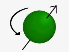
Figure 1. Graphical Representation of a Spin State as a Vector.

With this intuition, we should expect the rotation operator to be related to the angular momentum operator. For an internal rotation, the angular momentum operator is $\hat S$; for an orbital rotation, we will learn later that the angular momentum operator is denoted by $\hat L$. We use $\hat J$ to denote angular momentum operators in general. Now we can try to formulate a QM operator for rotations. Since we know that any arbitrary rotation is composed of an infinite number of rotations by an infinitesimal angle, knowing the expression for an infinitesimal rotation operator should lead us to the most general form of the rotation operator. The infinitesimal rotation operator is defined to be:

On the LHS, $i$ denotes the direction we are rotating in, and $d \phi$ is the angle we rotate through. On the RHS, we have $i$ denoting the complex number, and $\hat{J_i}$ denoting the angular momentum operator. Notice the correspondence between the direction of rotation and the subscript for the angular momentum operator.

There are three ways to check the validity of this definition.

1. The dimensions are preserved on the RHS. Indeed, angular momentum operators has the unit of $\hbar$.
2. $\hat{R_i}(d\phi = 0) = \pmb 1$, which is consistent with out expectation that rotation 0 degrees is equivalent to doing nothing.
3. The norm of an arbitrary state should be preserved when being acted on by the rotation operator. To verify this, we need to remember that calculating the norm of a state (no matter before or after applying the rotation operator) requires taking the inner product of the state by itself, and that the adjoint of an operator is just the complex conjugate.

Check that the rotation operator preserves the norm:

We can see that the norm is preserved up to $d\phi$ squared. Since the angles are infinitesimal, we can take the second order term to be much smaller than the first order terms, then the norm is preserved. If this explanation is unsatisfactory to you, remember that what we are looking at is just the infinitesimal rotation operator, not the rotation operator itself. Once we get to the “real” rotation operator, we will see that the norm is preserved without any approximations.

Now we need to find a way to go from the infinitesimal rotation operator to the “real” rotation operator. Remember that any rotation is achieved by rotation through an infinitesimal angle many times, and each infinitesimal rotation is mathematically achieved by multiplying the original state by the infinitesimal rotation operator. Thus, the full rotation operator should be a product of an infinite number of infinitesimal rotation operators! This sounds complicated, but writing it down makes things much clearer. Using the definition for the infinitesimal rotation operator we had before, change $d\phi$ to $\phi$, the total angle we rotate through, divided by $N$. Then take the entire thing to the $N$th power because we need to apply it on a state $N$ times. Finally, take the limit as N approaches infinity to go from finite to infinitesimal. We have:

Remember the definite of exponential of e, we can simplify this expression and get:

Now we finally have our rotation operator derived. More rigorously speaking, we have a set of three such rotation operators, each for one of the coordinate axes.

Notice that it obviously preserves the norm. (Check that yourself!)

The rotation operator looks a bit intimidating, but it’s action on a given state is actually very simple. As an example, let’s investigate the internal rotations of a spin-1/2 particle. Take the state $|+z\rangle$ and try to rotate it along the z-axis an angle of $\phi$. We have:

Utilizing the Taylor expansion of exponentials of $e$, we have:

This is a common way of handling operators in exponential forms. Once you are familiar with it, you can immediately write out the answer.

Angular Momentum Operators

Now that we understand the rotations in QM and the rotation operator, let’s turn our attention to the angular momentum operator $\hat J$. We first encountered the angular momentum in the expression for the infinitesimal rotation operator, and due to that expression, the angular momentum operator is also know as the generator of rotations. To better understand how bizarre angular momentum is in the QM context, we first need to learn a new mathematical tool called commutators.

In classical physics, we take for granted that a given object can have many different physical traits (e.g. mass, energy, momentum), and, more importantly, that we can know all these traits precisely at the same time. But if you think carefully enough, you will see that the postulates of QM implies that this is not necessarily true in the QM world. Making a measurement of an observable in QM is equivalent to applying an operator on a state, and no one can guarantee that this state remains unchanged afterwards. In fact, only when a state is a degenerate eigenstate of the operator, the state is guaranteed to be unchanged. Therefore, it is possible that measuring one physical quantity perturbs the particle’s state such that other quantities cannot be known at the same time. Commutators can help us determine whether two physical quantities can be measured at the same time or not.

Commutator is an operation that takes in two operators and outputs another operator (which can be zero). Mathematically it is written as:

When the commutator of two operator is equal to zero, the two corresponding physical quantities can be known at the same time. When the commutator is not equal to 0, the two physical quantities cannot be known at the same time. More specifically, the uncertainties of these two quantities are given by:

where $\Delta A = \langle \langle A \rangle - A \rangle$ is the standard deviation of the measurement of $A$. This is known as the generalized uncertainty principle (proof).

It’s rather involved to derive the commutators of the angular momentum operators using the rotation operators, and we will give the relationships for now:

And cyclic permutations.

This is a very counter-intuitive result! What this is telling us is that we cannot know two different components of the angular momentum of a particle at the same time. However, we can define the total angular momentum operator $\hat J$, which satisfies:

We can derive that :

To sum up, somehow we are able to know the magnitude of the angular momentum and one of its components at the same time, but nothing more. A further implication of this result is that the angular momentum of a particle cannot be parallel to any one of the coordinate axes. If that were true, we would be able to know all three components at once (the angular momentum along the two other axes were zero).

As implied above, if two operators commute, they share the same eigenstates, so that we can label a quantum mechanical state as a combination of their eigenstates. After knowing all these information, we have a new way of labelling a quantum mechanical state. According to conventions, we choose to use the angular momentum along the z-axis and define the eigenvalues of the two commuting operators as:

where $m$ is the eigenvalue of $\hat{J_z}$, while $j$ is more mysterious and the eigenvalue of $\hat J^2$ is $j(j+1)$. In other words, $\sqrt{j(j+1)}\hbar$ represents the measurement of total angular momentum. In order to explain the significance of $j$, we define a new set of operators from the angular momentum operators and see what effect they have on a given state:

Let’s calculate the following commutator, which happens to be really useful,

Then act $\hat{J_z} \hat{J_\pm}$ on $|j, m\rangle$ with this relationship in mind,

We somehow obtain the eigenvalue corresponds to the eigenstate $|j,m\pm1\rangle$! This suggests that

where $c_\pm$ is a complex number and $\hbar$ preserves the units.

The two new operators are called raising and lower operators. As I just showed, their effect is to raise or lower the z-component of the angular momentum by $1$. Hence the name. Physically, the z-component of the angular momentum cannot increase or decrease indefinitely, as we expect its magnitude to be less than the total angular momentum $\sqrt{j(j+1)}\hbar$.

Let the maximal $m$ value be $m_{max}$, then $\hat{J_+} | j, m_{max}\rangle = 0$. We first calculate the useful relationship below:

Then apply the relationship,

Now we see that $j=m_{max}$. With a similar derivation, we can see that $-j=m_{min}$

For orbital angular momentum, we use $l$ for $j$, and $m_l$ for $m$. For intrinsic angular momentum, i.e. spin, we use $s$ for $j$, and $m_s$ for $m$. When we we talk about spin-1/2 particles, we are actually saying that $s = 1/2$! Now you know why spin-1/2 particles have only two states:

For a particular $j$, the range of $m$ is within the range from $-j$ to $+j$ and takes steps of $1$. When you hit the smallest $m$ value state with a lowering operator or hit the largest $m$ value state by a raising operator, you simply get $0$. According to research in the field, we know that $j$ can only be integers or half integers.

Matrix Representations of Angular Momentum Operators

It will be very convenient to find out the matrix representations of the angular momentum operators, so that we can derive the eigenstates and the eigenvalues. We will try to find the representations of the operators in z-basis. For $J_z$, it is simple, as it is the diagonal matrix with the eigenvalues of each eigenstate on the diagonal. For example, we already know that for a spin-1/2 particle, the eigenvalues are $m_s = \frac{1}{2} \hbar, -\frac{1}{2} \hbar$

Similarly, for a spin-1 particle the eigenvalues are $m_s = \hbar, 0, -\hbar$,

But it is harder to get the anglar momentum operators with the other two directions. Luckily, we have $\hat{J_\pm} = \hat{J_x} \pm i\hat{J_y}$, so all we need to do is to find $\hat{J_\pm}$ in the z-basis.

We already have that:

And that:

We can also show that the raising and lowering operators are the adjoint of each other:

Now we can obtain:

Assuming the angular momentum states satisfy $\langle j, m|j, m\rangle = \langle j, m+1|j, m+1\rangle$, we can choose

Similarly, we can derive

For an angular momentum space with basis states $|x_i\rangle$, we can calculate the $(ij)$th component of the matrix representation of $\hat{J_\pm}$ by $\langle x_i|\hat{J_\pm} |x_j\rangle$. This shoud be apparent with some study of linear algebra.

Now let’s take the spin space of spin-1/2 particles as example, which has the basis states

With some calculation, you can check that:

Now we can easily write out the matrix representations for the spin operators:

These matrices, without the factors of $\frac{\hbar}{2}$, are known as the Pauli spin matrices.

We can now derive $|\pm x\rangle$ and $|\pm y\rangle$ as promised in the first post by calculating the eigenstates of $\hat{S_x}$ and $\hat{S_y}$:

We can also represent the rotation operator with a matrix. A bit of mathematics: If A is a matrix, then the exponential of A is given by:

This result is hard to prove. For non-diagonal matrices, exponentiating becomes very painful. I will not go into too much details here and leave the proof to the mathematicians. What’s important for us is to use this result to obtain the matrix form of $\hat{R_z}$ for the internal rotation with $\hat{S_z}$:

References

[1] Zajc, William. PHYS GU4021-4022 Quantum Mechanics I-II, Department of Physics, Columbia University. 2019-2020.

[2] Townsend, John. A Modern Approach to Quantum Mechanics. 2nd Edition.