We are quite familiar with the idea of quantum mechanical states now. However, all the states we’ve been dealing with are states of only 1 particle. It’s time to extend our discussions to the states of 2 particles.

2-particle systems

Remember from before that the quantum mechanical state of a particle resides in its own Hilbert space. Extending this idea to 2 particles, we say that each particle has its own Hilbert space. Notionally, we can use subscripts under the bra and ket symbols to distinguish between different Hilbert spaces. For example, states of particles 1 and 2 can be written as: $| \psi \rangle_1$ and $| \phi \rangle_2$ Where $\psi$ and $\phi$ are two single particle states and the subscripts “1” and “2” denotes two different Hilbert spaces. In all previous posts, we’ve been exploring how to manipulate these states individually, but now, we want to find a way to “unite” the 2 particles as a whole. The formal mathematically way of achieving this is called a tensor product. A tensor product is an operation between Hilbert spaces, by taking the tensor product of 2 single particle states, we get a new 2-particle-state:

Don’t worry if all of this sounds abstract. The main takeaway here is that we can write a 2-particle-state as a tensor product of two single particle states, but at the same time, we need to be clear that each particle has its own Hilbert space, which means it can only be acted upon by operators in its own Hilbert space. So how do the operators behave? Suppose we have two operators $\hat O_1$ and $\hat O_2$ that measures the same observable and belongs to Hilbert spaces 1 and 2, respectively. Let’s try to apply them on our new 2-particle state and see what happens. Keeping in mind that operators are only effective on states in its own Hilbert space, we have:

Just like we have a new state as the tensor product of two single particle states, we also have a new operator for the sum of two “single particle operators”, $\hat O = \hat O_1 + \hat O_2$:

Example: two spin-1/2 particles

Now let’s look at a more concrete example to consolidate our understanding. Consider the spin state of two spin-$\frac{1}{2}$ particles (say, two electrons). First, let do some review on notation, specifically on how to label a spin state. In the second post, we discussed how to label the spin state of a particle by the two quantum numbers: $s$ and $m_s$, where $s$ is the total spin, and $m_s$ is the spin along the z-axis (by convention). For the two spin-$\frac{1}{2}$ we are dealing with here, they can only be in one of these two states:

We know the behavior of these states pretty well now, but things become more complicated when we consider the two-particle states. Knowing that each particle can be either spin up or spin down, we should have a total of four possible two-particle states. Let’s examine these states more closely.

To understand what’s going on for each of the two-particle states, the easiest way is to find its angular momentum on the z-axis. We are applying an operator on a two-particle state, so we should be using the “total” $\hat S_z$ operator:

Using the rules we discussed before, we have:

Similarly, we have:

We see that the eigenvalues, which are the angular momentum values, are $\hbar$, 0, and $-\hbar$. This should immediately remind you of the behavior of spin-1 particles. However, there is a crucial difference: there are four two particle states here and a twofold degeneracy at the eigenvalue of 0, but spin-1 particles should only have 3 different spin states. To resolve this, we introduce what’s called a spin-0 state, which has a single eigenstate with the eigenvalue $0$.

Using the $|s, m_s\rangle$ notation, we have a spin-1 triplet:

and a spin-0 singlet:

From this point on, I’m going to leave out the tensor product symbol. Most of the times it’s safe to assume it as just a normal product.

It’s easy to distinguish the states with angular momenta $\hbar$ and $-\hbar$:

But how do we assign $|1,0 \rangle$ and $|0,0 \rangle$ to the states $| \frac {1}{2},\frac {1}{2} \rangle_1 | \frac {1}{2},-\frac {1}{2} \rangle_2$ and $| \frac {1}{2},-\frac {1}{2} \rangle_1 | \frac {1}{2},\frac {1}{2} \rangle_2$ given that they have the same eigenvalues? The answer lies in the raising and lowering operators we introduced in the second post. We can always generate the $|1,0 \rangle$ state by applying the raising operator to the lower state $|1,-1 \rangle$, but the same doesn’t hold for $|0,0 \rangle$. Let’s make full advantage of this difference.

First recall the most general behavior of the raising operator:

So when $s=1$ and $m_s=-1$, we have:

Now, we know the LHS of this equation very well. Just be careful: the $\hat S_+$ operator is the “total” raising operator. We have:

Which means:

and correspondingly:

In summary, a system of two spin-1/2 particles behaves like a spin-1 triplet and a spin-0 singlet. We can actually summary all of this section into one equation: $2 \otimes 2 = 3 +1$. It shouldn’t be a surprise that for the two-particle system of a spin-1 particle and a spin-1/2 particle behaves like a spin-3/2 particle and spin-1/2 particle: $3 \otimes 2 = 4 +2$.

Hydrogen Atom and the Hyperfine Splitting

You might be wondering why we choose a system of two spin-1/2 particles in our analysis above. One of the answers is that the most abundant element in the universe, hydrogen, is essentially such a system: Protons and electrons are both spin-1/2 particles. Using what we just learned, let’s try to find the energy levels due to the spin-spin interaction of the proton-electron system in an hydrogen atom.

We know that both a proton and an electron have magnetic dipole moments, and the particles in an atom will experience magnetic interactions. We will restrain our discussions to the ground state of a hydrogen atom, which means the orbital angular momentum is $0$ and spins of the particles are the only sources of the magnetic moments. We can then relate the interaction Hamiltonian to the spin operators of the proton and the electron.

where $A$ is a constant, and I changed electron and proton to $1$ and $2$, respectively, for convenience. So have do we find the eigenvalues of this interaction Hamiltonian expressed as a dot product of two spin operators? It is convenient to utilize the total spin operator here:

So we have:

Now, we know that for $\hat{S_1}$ and $\hat{S_2}$, the eigenvalue $s = \frac {1}{2}$. But for $\hat{S}$, the total spin operator, there are two possible eigenvalues, $0$ and $1$, that corresponds to the spin-1 triplet and the spin-0 singlet. So we have two eigenvalues for the interaction Hamiltonian. This is what’s called the hyperfine structure of the ground state of the hydrogen atom.

Carrying out the relevant calculations, we get the two eigenvalues to be $\frac {1}{2} A$ and $-\frac {3}{2} A$. This energy difference of transition from triplet to singlet has been measured to correspond to a wavelength of 21 cm. In astronomy, this is known as the 21-cm H line.

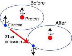
Figure 1. The 21-cm H line as the result of a change in total spin. (Image source: Cosmic Glimpses)

The EPR Paradox

Now let’s switch gears a bit a look at a counter-intuitive experiment that illustrates some of the essence of QM. Let’s start with the spin-0 singlet state of two particles. Suppose it decays into two spin-1/2 particles that travels in opposite direction. At the same time, two physicists, Alice and Bob, are opposite sides of where the decay happens. Each of them have a Stern-Gerlach apparatus that measures the spin of a particle.

By conservation of angular momentum, we know that the angular momenta of the two particles that comes out of the decay should sum to $0$. In QM, we say the two particles are in an “entanglement”. In plain English, this just means that there is a definite relationship between some characteristics of the two particles. In our case, it’s the angular momentum of the particles that’s “entangled”. From a more practical standpoint, we can define “entangled states” as states that cannot be written as a simple product of two single-particle states.

Before any measurement is made, the spins of the two particles are indeterminate, meaning that they can have angular momentum of $\pm \frac{1}{2}$ along any axis as long as the total angular momentum sum to 0. Now suppose Alice makes a measurement of angular momentum along the z-axis and gets a result. At the same time, she can also immediately deduce the result of Bob’s measurement using the law of conservation of angular momentum. This all seems nice and logical, right?

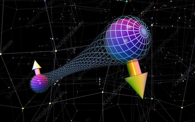
Figure 2. The EPR paradox: quantum entangled particles. (Image source: Russell Kightley - Science Photo Library)

Some physicists, including Einstein, Podolsky, and Rosen are skeptical about this scenario, and they raise this though experiment known as the EPR paradox. In particular, they pointed out that if Alice and Bob are separated by some finite distance, it is impossible for Alice to know Bob’s measurement results immediately. This instantaneous transmission of information violates the principle that no information can travel faster than the speed of light. As a result, physicists like Einstein claims that there must be some intrinsic property of the particle that determines the results of the measurements. These properties are within the particles as soon as they are produced from the decay, so the measurements actually give us no new information, and nothing travels faster than the speed of light. Due to this point of view, these physicists are also know as “objective realists”, and the theory a “hidden-variable theory”.

The view of the objective realists might sound tempting and consistent with our intuition, but QM never ceases to challenge our intuition. Bell’s theorem and related experiments prove that QM is incompatible with a hidden value theory. Many more experiments have demonstrated again and again that the objective realists are wrong, and that the measurements produce results that cannot be predicted or known in any way.

But does this mean that some information traveled faster than the speed of light when the measurements are being made? The answer is no! The information about the entanglement of the two particles are “communicated” when the decay happened. It’s like giving your mom a letter with your screwed-up QM exam in it, then your mom opening the letter a light year away and immediately knowing the fact: The information is communicated when you gave the letter. Of course, the analogy is flawed and isn’t counter-intuitive as quantum entanglement at all. Nonetheless, this experiment is perfectly self-consistent and can be explained well by QM. If you still think there is a paradox somewhere, then you must be still in the mindset of object realists.

The Density Operator

For now, we are purely dealing with single system states, or pure states. But in the real world, a mixture of particles almost always resemble a mixture of states, therefore a mixed state.

The main function of the density operator is that it helps us distinguish between pure states and mixed states and allows simpler calculation of quantities like expectation values.

We will be dealing with (systems of) spin-1/2 particles only, so I will use + and - for spin up and spin down for convenience.

Here’s how we go from a state to a density operator of that state:

And of course, we can use the conventions of matrix mechanics to express it as a matrix.

All the states we’ve been expressing using the bra-ket notation are “pure states” and can be easily transformed into density operators. At the same time, density operators can also express mixed states. For example:

represents a 50%-50% mixture of spin up and spin down particles.

In matrix form, the density operator offers us many “shortcuts”. The trace (sum of the diagonal elements) of density operators is always 1. The trace of the density operator squared is 1 for pure states and <1 for mixed states. (try to verify this by yourself)

To calculate the expectation value of physical quantities, we just need to transform the corresponding operator into matrix form and use:

References

[1] Zajc, William. PHYS GU4021-4022 Quantum Mechanics I-II, Department of Physics, Columbia University. 2019-2020.

[2] Townsend, John. A Modern Approach to Quantum Mechanics. 2nd Edition.