Why is Sky Blue?

Why is sky blue? You may know the answer is Rayleigh scattering. But how do we understand Rayleigh scattering? We will try to find the answers in Maxwell’s equations and a simple dipole model.

Recap on E&M

All easy questions can be extremely hard if you keep asking the questions. “Why is sky blue”? “Because blue light, which has larger frequency, scatters more.” One might answer. “But what causes the scattering and why is there a frequency dependence?” For this post, we will find the answer from Maxwell’s equations.

Witht the right Gauge transformation (Lorentz Gauge), we have the clean potential equations

where $\square^2 = \nabla^2 - \frac{1}{c^2} \frac{\partial^2}{\partial t^2}$.

If the potential is not time-dependent, we recover the Poisson equations, for which the solutions are

where $\rho$ is the charge density, $\mathbf{J}$ is the current density.

For the full time-dependent equations, the solutions look very much like the above, but the charge and current density are evaluated at the “retarded time” $t_r$.

where $t_r = t - \frac{\|\mathbf{r} - \mathbf{r}'\|}{c}$. This manifests the causality: the information that the densities changes cannot propagage faster than the speed of light.

For fun but not really related to our main discussion, we will digress and derive the potentials for a point charge $q$ with a trajectory $\mathbf{w}(t)$. The potential equation reduces to

where $\mathbf{s} = \mathbf{r} - \mathbf{w}(t_r)$.

The potential looks very similar to a static charge,

But again, due to causality, or the relativistic effects, we see the manifest of length contraction with the $1-\hat{\mathbf{s}} \cdot \mathbf{v}(t_r)/c$ factor. The retarded time is implicitly defined by

Similarly we have that

Radiation

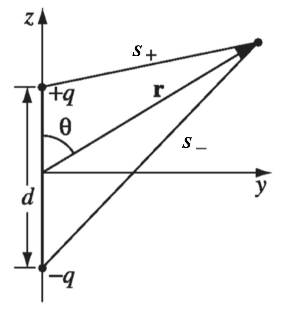
Now we are finally in good shape to talk about radiation. In essence, radiation is the emission of energy by moving charges. Moving charges cause a change in the fields, which causes EM waves, which propagates energy. In the case of the atmosphere, the interaction between sunlight (radiation from the nuclear reactions of the sun) and the charges in the atmosphere. As a simplified model (which turns out to succesffully explain the color of the sky), we will assumes the charges oscillate like a electric dipole, i.e., two opposing charges $q(t)$ and $-q(t)$ are held $d$ apart, where $q(t) = q_0 \cos(\omega t)$. This may seem a bit unphysical, and an equivalent picture of the system is when the two opposing charges $q_0$ and $-q_0$ are connected by a spring which oscillates with frequency $\omega$, but this will make calculations a bit more complicated.

where $s_{\pm} = \sqrt{r^2 \mp r d \cos \theta + \left(\frac{d}{2}\right)^2}$.

Our next step is to make some physical approximations. To start with, we will assume that the separation between the charges are very small. How small? (1) $d<<r$, i.e. we are only worried about the field sufficient far away; (2) $d << \frac{c}{\omega}$ or $d << \lambda = \frac{2 \pi c}{\omega}$, i.e. the separation is small compared to the wavelength of the oscillation. Thus, the potential can be simplified into

Now at the limit of $\omega \rightarrow 0$, the second term reduces to the potential of stationary charge. However, the second term will not survive due to the $1/r$ dependence, and thus is not of the interest for radiation. We are interested in the range of (3) $r >> \frac{c}{\omega}$, in which case potential reduces to

We can similarly calculate the vector potential $\mathbf A(r, \theta, t)$, and with Maxwell equations and the approximation at large $r$, we can find the EM fields:

The energy radiated by an oscillating electric dipole is determined by the Poynting vector:

The intensity of the emitted light is obtained by averaging (in time) over a complete cycle:

Now it’s easy to see that the intensity depends on the frequency $\omega$ at its 4th power. Thus, the higher the frequency, the larger the intensity. And Voilà! Among the colors most sensitive to our eyes (blue, red, green), blue light has the largest frequency.

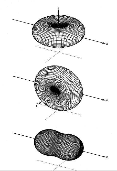
It’s curious to note also that the intensity has a $\theta$ dependence. In particular, the intensity is $0$ when $\theta = 0$. Since EM waves are transverse, the dipoles oscillate in a plane orthogonal to the sun’s rays. This means that when the eye of sight is perpendicular to the sun’s rays, $\theta=0$ and we should not see any radiation! But this is of course not true based on our observation. Our model accounts for a polarized EM wave which induces a particular dipole direction. However, sun’s rays are unpolarized and consist of a mixture of polarization directions. In effect, we can reduce any direction to a linear combination of two axis-aligned directions, and each polarized ray produces intensity as calculated which looks like a donut (top two plots below). And for an unpolarized light, the distribution can be obtained intuitively by rotating a polarized distribution around the axis of propogation of light (bottom plot below), results in a $(1+cos^2 \theta)$ dependency instead, which is correctly characterized by Rayleigh scattering.

Now you can always ask further where does Maxwell’s equations come from, but unfortunately the discussion will end here today.

References

[1] Zajc, William. PHYS GU4021-4022 Quantum Mechanics I-II, Department of Physics, Columbia University. 2019-2020.

[2] Griffiths, David. Introduction to Electrodynamics. 4th Edition.

[3] Petty, Grant W.. A First Course in Atmospheric Radiation. 2nd Edition.