Word2Vec
June 10, 2020
This post introduces some methods to create vector embeddings for words that are/were widely used: Skip-Gram, CBOW, and GloVe.
When solving any real-world problems with computer algorithms, one crucial to consider is how to represent real-world data with bits and bytes. In the field of language processing, our major concern is words. How to efficiently represent words?
This post is based on the lectures of Stanford cs224n (2019 Winter).
One-hot vector
Perhaps the most intuitive way is to simply label each work with a unique number. Say our vocabulary is:
['I', 'want', 'to', 'represent', 'words']
We can define a look-up table pairing up each work with a unique index:
| Word | Representation |
|---|---|
| I | 1 |
| want | 2 |
| to | 3 |
| represent | 4 |
| words | 5 |
We assign each word an index . But this embedding scheme has several disadvantages. (1) Since each has a different magnitude, which signifies words have importances. (2) Also, of different words have no correlations between their meanings. Ideally, we want for embeddings for correlated words to also have correlated representations.
The first problem can be solved by representing words with one-hot vectors. We represent each word with a vector , where is the vocabulary size. Every entry of is zero except that the i-th entry is one. So now for our mini vocabulary we have:
| Word | Representation |
|---|---|
| I | |
| want | |
| to | |
| represent | |
| words |
This solves the problem (1) and offers us vectors to work with, which is pretty convenient. But the problem (2) remains. Moreover, we now have a problem (3): the curse of dimensionality. With a small this is still viable, but imagine trying to incorporate all possible words we have using this representation…
Word2Vec
This motivates a vector representation of words with smaller dimensionality vectors and some kinds of correlations with their meanings.
Suppose each word is represented by some vector , where is the embedding size, a ‘small’ number. We can make use of dot product to measure how close two vectors are. So ideally, if and are correlated, will be big (close to 1). Conversely, if and are not correlated, will be small (close to -1). We will take this as a basis of intuition when we measure correlation in the following derivations.
Before that, you may notice that ‘correlated’ is ill-defined here. It can mean that two words are close in meanings, or it can mean that two words often appear together. The two interpretations sometimes align, but we need to treat them differently. The two algorithms I will introduce, Skip-Gram and CBOW, use the second definition.
The idea behind both algorithms is simple. We want our vector embeddings of correlated words and to produce high conditional probability .
-
Question 1: how do we know and are actually correlated?
Answer: we find many real sentences and see what words are presented together. In reality, a sentence can be arbitrarily long, and we take a sliding window approach. For a sliding window of size , we only look words coming before or after a word.
-
Question 2: how do we measure ?
Given the intuition about the dot product above, this should somewhat make sense. Dot product measures the correlation; by taking the exponentials, we pick out the bigger values and normalize all the values to sum to one to make a probability distribution. This comes from a cross-entropy loss and softmax function (more on this later).
CBOW (Continuous Bag of Words)
Given a center word , we refer to the words around as the context words for . CBOW seeks to maximize the probability of having a center word its context words within a particular window size , so there are context words ( words on the left and on the right) for a center word. (The center words at the beginning or end have fewer context words.) To make the algorithm easier in practice, we often assign two vectors to each word , one vector for the word when it is a context, and the other when it is a center word. In the end, we average out the two vectors. You will see how this will simply implementations.
In short, for a single center word, we want to maximize:
We haven’t talked about how to model the probability of a word given many words. CBOW takes a rather straightforward approach. We average out the word vectors of the words and conditioned on that averaged value instead.
Equivalenty, we want to minimize the negative log probability:
where
If we concatenate all vectors together, we get a matrix , where is the vocabulary size and is the embedding size or the dimension of each word vector. The ith column of is for word . Similarly, we have a for all . Now we again find one-hot vectors extremely useful. For a word with one-hot vector , we get and . This is non-trivial as it enables a vector-based implementation (without nasty for-loops). More importantly, this gives another interpretation of other than the concatenation of vectors: they can be understood as two weight matrices to be learned.
Now we have some vector representations, some probability models, and some loss functions, and some weights to be learned. It should be clear now this is a standard machine learning problem.
Algorithm
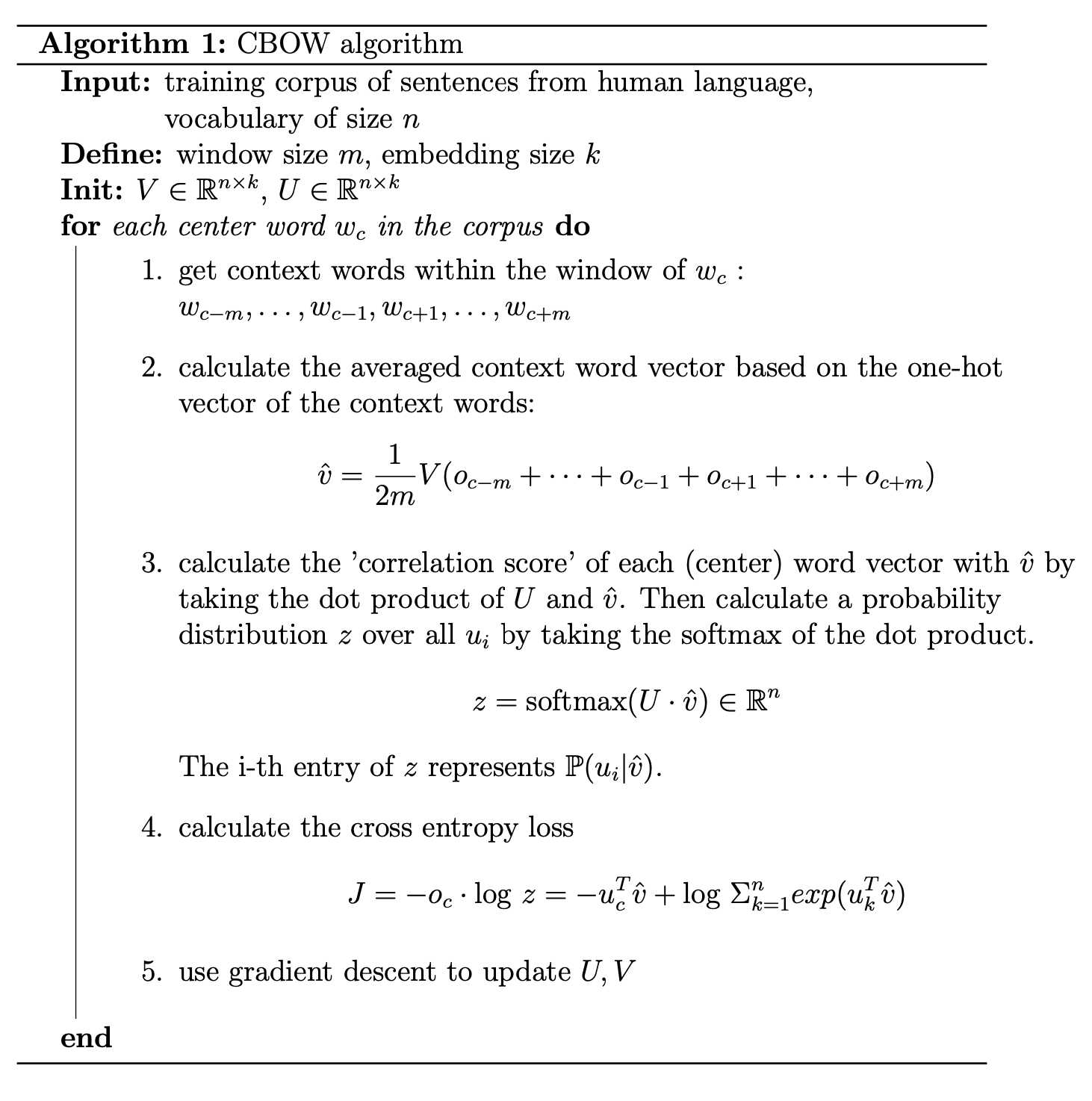
Previously we get the loss from the negative log probability, but we didn’t explain how we get that probability (though we use the intuition of dot product to infer it). The steps 3 and 4 explain how we get the loss from a softmax function and cross-entropy loss. You may need to write out the equations to see how they equate. Another thing to mention is that in practice, we take a gradient step for several center words instead of a single word as it may imply.
Skip-Gram
Skip-Gram is very similar to CBOW. Instead of considering the probability of a center word given some context words, Skip-Gram seeks to maximize the probability of context words given a center word.
To do gradient descent, we need to calculate partial derivatives of w.r.t. . For a single context word :
This is actually intuitive, since with each update,
we are essentially pushing towards with discount of that already has large with some learning rate .
where is the indicator function.
Negative Sampling: The Problem with Softmax and Solutions
To get a probability distribution over every word (given a center word or some context words), we need to calculating softmax. But this can be problematic, as again we need to output an entry for every word in the vocabulary. To avoid the curse of dimensionality, there are two widely-used approaches: Negative Sampling and Hierarchical Softmax ([2]). This post will breifly introduce negative sampling, and you may look up hierarchical softmax for further exploration.
Rather than directly optimizing a conditional probability where is a pair of word that appears together, negative sampling seeks to train a classifier that predicts whether is a valid pair. For example, (“play”, “game”) appears to be valid and we want the classifier to predict true, while (“eat”, “game”) appears nonsensical and we want the classifier to predict false.
During the training, the validity of a pair is defined as whether the pair appears in the corpus data . We will denote by the probability of coming from , and vice versa, where is the parameters of the model which in this case are the word vectors and .
We model this probability with the sigmoid function of the dot-product between word vectors:
We train our model by taking a maximum likelihood approach:
where is assumed to be some “false” corpus which contains nonsensical word pairs. But we don’t really have such a corpus, and we will model such a “false“ corpus by randomly sampling times from a probability distribution given a word .
Thus, given a true word pair , a center word and a context word, seen in the corpus data, we can define a loss function by nagative log likelihood:
where .
The researchers have found that the unigram distribution (the distribution based on each word’s frequency) raised to 3/4rd power has the best performance:
where is a normalization factor.
GloVe (Global Vectors for Word Representation)
Both CBOW and Skip-Gram have problems of locality: We are attending to co-occurred words within a limited window size. What if we want to make use of global cooccurrence? Suppose we have a global cooccurrence matrix , where represents the cooccurrence number of words and . How can we make use of them?
Another idea is that we don’t just want some conditional probability . Instead, we want some comparative measure of
GloVe is motivated by the ideas of using global cooccurrence and the need to represent a relative cooccurrence. For words and their corresponding vectors , (every word again has two vectors), we model the conditional probability as:
Now we have a nice property of:
We define the loss function :
where is some clipping function that clips large , and are biases.
References
[1] Mikolov et, al. Efficient Estimation of Word Representations in Vector Space. (CBOW and Skip-Gram)
[2] Mikolov et, al. Distributed Representations of Words and Phrases and their Compositionality. (negative sampling and hierarchical softmax)
[3] Penning et, al. GloVe: Global Vectors for Word Representation. (GloVe)