From Sequence to Attention

June 14, 2020

This post gives a gentle introduction to the neural models used in NLP in recent years, which sees a trend from sequence models (RNN, GRU, LSTM), to attention-based models (transformers).

Sequence Models
Transformers (Hail to Self-attention!)
References

Sequence Models

Sequence models, as the name suggests, process a sequential data in sequence. This seems particularly suitable for natural language, as we humans speak, read, write in sequence. It seems reasonable for machine learning models to process language in sequence as well. In deep learning, sequence models are usually based on recurrent neural networks (RNN)

Vanilla RNN

The diagram below illustrates the structure of RNN models. The red blocks represent the inputs in sequence from left-to-right. The blue blocks are the outputs, also produced in sequence. The green blocks are the hidden states of the model, which is produced by running the current input (red block below) and the last hidden state (green block on the left) though some neural network.

For different tasks, we produce different numbers of outputs. For example, for sentiment analysis, we use a “many-to-one” RNN, which predicts the sentiment of a sentence based on the very last hidden state which should encapsulate the semantics of the entire sentence. For Language Modelling (LM), which is to produce the next word based on previous words, we use a “many-to-many” RNN.

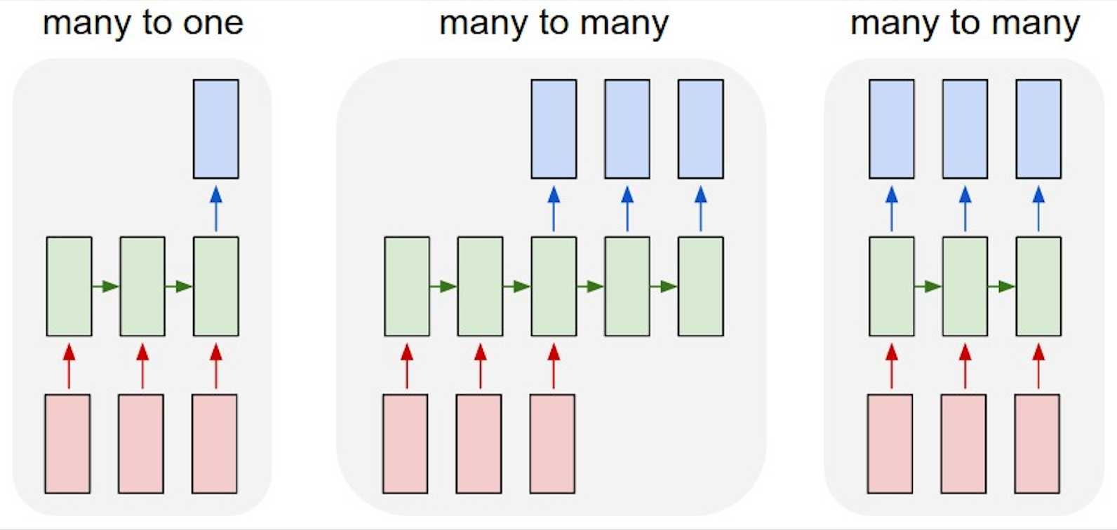Figure 1. Different types of RNN. (Image source: Andrej Karpathy blog)

LSTM

RNN has a huge problem with vanishing/exploding gradients. For each hidden state, we are essentially using two same weight matrices $\mathbf{W_x}, \mathbf{W_h}$ and apply them to the previous hidden state $h_{t-1}$ and current input $x_t$ to produce $h_t$ . During the backward pass, when calculating the gradient w.r.t. the hidden states far away at the beginning, we multiply the weight matrices multiple times, which will produce a vanishing or an exploding gradient depending on the “magnitude” of the matrices. For vanishing gradient problem, it means that gradient signals from faraway are much smaller than gradient signals from close-by, and therefore the weight updates will tend to be influenced by states close by. In the context of a language model, this means that the generation of the next word is heavily influenced by the previous word as opposed to words at the beginning, which is not always optimal.

This problem motivates the development of LSTM as illustrated below. The essential idea is that the current hidden state may not be closely related to the previous hidden state; it may be more closely related to some hidden states faraway. In order to keep the information from the beginning, we keep a cell state in addition to the hidden state as a memory. There are a lot of great posts that give much more detailed explanations of LSTM, for example Understanding LSTM Networks), where I took the picture below. Please check out those sources for a thorough introduction to LSTM.

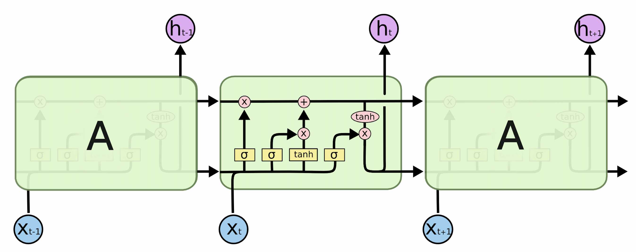Figure 2. LSTM. (Image source: Understanding LSTM Networks)

For the vanilla RNN,

h_t = \sigma (\mathbf{W_x} x_t+ \mathbf{W_h} h_{t-1} + b)

where $b$ is the bias.

For LSTM, we have 3 gates and 2 states. Each gate is like a continuous switch and has values from 0 to 1. The 2 states are the cell state $c_t$ , which is kind of like a memory, and the hidden state $h_t$ , which is used to produce some outputs like the hidden state in vanilla RNN.

3 Gates of LSTM

Variable	Significance	Expression
Forget gate $f_t$	Controls how much of the previous cell state $c_{t-1}$ content will be remembered in the new cell state $c_{t}$ .	$f_t = \sigma (\mathbf{U_f} x_t+ \mathbf{W_f} h_{t-1} + b_f)$
Input gate $i_t$	Controls how much of the new cell content $\tilde c_{t}$ (see below) will be wrote to the new cell state $c_{t}$ .	$i_t = \sigma (\mathbf{U_i} x_t+ \mathbf{W_i} h_{t-1} + b_i)$
Output gate $o_t$	Controls how much of the new cell state $c_{t}$ will be wrote to the hidden state $h_{t}$ .	$o_t = \sigma (\mathbf{U_o} x_t+ \mathbf{W_o} h_{t-1} + b_o)$

2+1 States of LSTM

Variable	Significance	Expression
Cell content $\tilde c_{t}$	Temporary values that quantify the new input into the model.	$\tilde c_{t} = \text{tanh } (\mathbf{U_c} x_t+ \mathbf{W_c} h_{t-1} + b_c)$
Cell state $c_{t}$	Remeber some content from the previous cell state and write some new cell content.	$c_{t} = f_t \circ c_{t-1} + i_t \circ \tilde c_{t}$
Hidden state $h_{t}$	Output some content from the new cell state.	$h_{t} = o_t \circ c_{t}$

GRU

Another model that is based on RNN, Gated Recurrent Units (GRU), has a very similar idea with LSTM but has simpler gate structures which results in efficiency in computation.

2 Gates of GRU

Variable	Significance	Expression
Update gate $u_t$	Controls how much of the previous hidden state $h_{t-1}$ will be erased in the new hidden state $h_{t}$ and how much of the new hidden state content $\tilde h_{t}$ (see below) will be updated.	$u_t = \sigma (\mathbf{U_u} x_t+ \mathbf{W_u} h_{t-1} + b_u)$
Reset gate $r_t$	Controls how much of the previous hidden state $h_{t-1}$ will be used to compute the new hidden state content $\tilde h_{t}$ (see below).	$r_t = \sigma (\mathbf{U_r} x_t+ \mathbf{W_r} h_{t-1} + b_r)$

1+1 States of GRU

Variable	Significance	Expression
hidden state content $\tilde h_{t}$	Temporary values that quantify the new input into the model.	$\tilde h_{t} = \text{tanh } (\mathbf{U_h} x_t+ \mathbf{W_h} (r_t \circ h_{t-1}) + b_h)$
hidden state $h_{t}$	Reset some content from the previous hidden state and update with some content from the new hidden state content.	$h_{t} = (1-u_t) \circ h_{t} + u_t \circ \tilde h_{t}$

Application: Seq2Seq NMT

Besides language modeling, sequence models have become very useful for machine translation tasks. Sequence-to-sequence Neural Machine Translation (Seq2Seq NMT) has been very successful. The basic architecture is an encoder-decoder pair, where the encoder gives a representation of a text from the source language, and the decoder generates a text from the target language based on the representation from the encoder. The decoder is essentially a language model that takes in the representation of the target text as a context.

The diagram below taken from Stanford CS224n illustrates the basic structure of Seq2Seq NMT. An additional component is the attention, which gives the decoder the additional capacity to selectively take in hidden states of the encoder as the input. Without the attention mechanism, the decoder can only generate outputs based on the encoder’s last hidden state, which is quite limited. As we translate a sentence, we often translate word by word, so we’d like to attend to a specific word from the source text when doing the translation. The attention mechanism is based on this idea. During each decoding step, the model takes a dot-product of the decoder embedding with all encoder hidden states and use the resulting values to produce a probability distribution over the encoder the hidden states (using softmax). Then a weighted average of the encoder hidden states based on the distribution is appended to the decoder embedding.

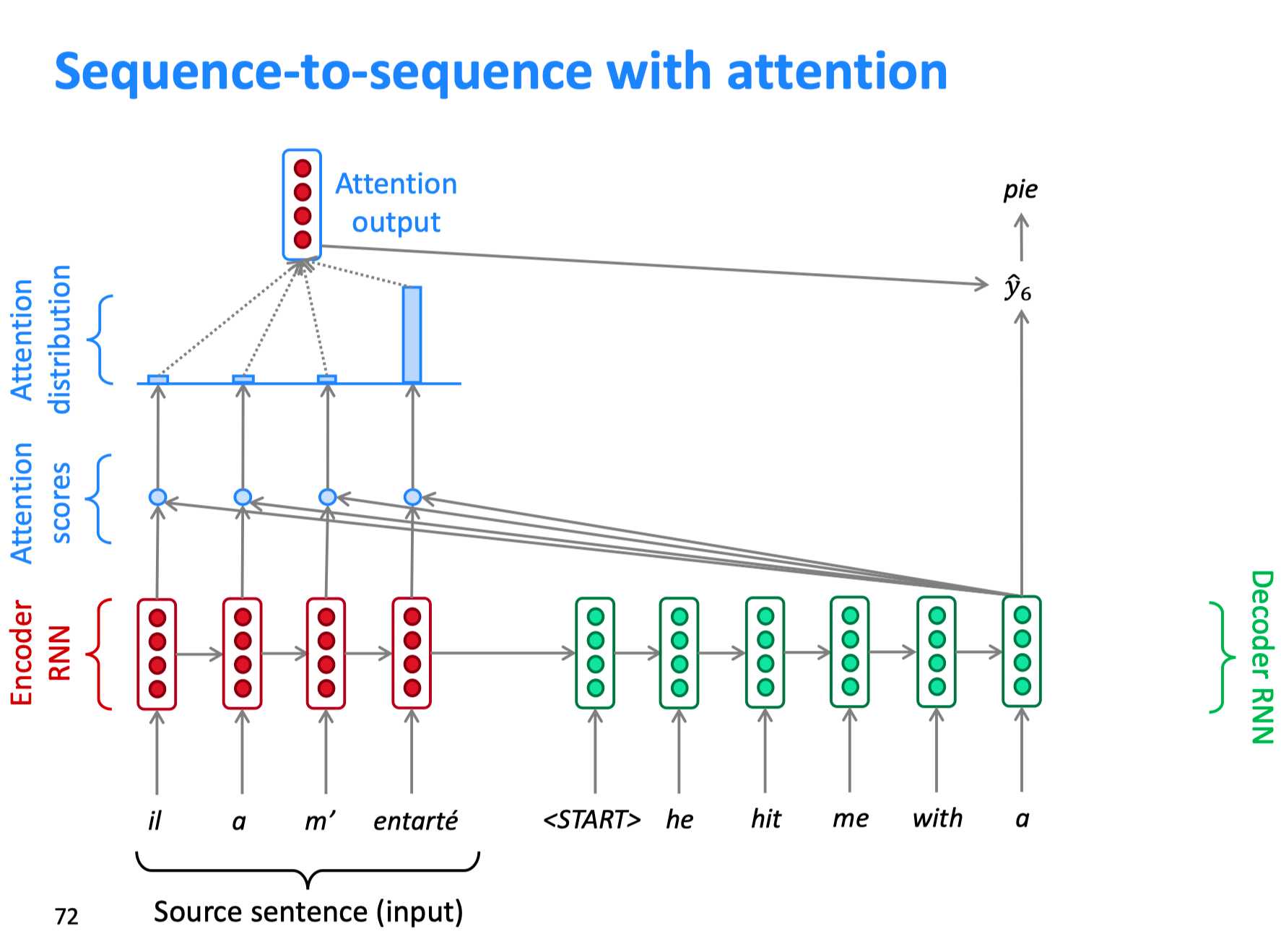Figure 3. sequence2sequence NMT. (Image source: Stanford cs224n Winter 2019 lecture 8)

Transformers (Hail to Self-attention!)

We’ve introduced the attention mechanism that significantly improves the performance of sequence models like seq2seq NMT. In fact, attention is a mechanism that can be applied to any neural network model. More obstructively, attention refers to a neural network’s ability to make inferences by selectively taking into account some data other than its inputs depending on some weights that can be learned. Data is referring not only to the raw data at the beginning but also any values produced by the model, such as word embeddings, intermediary encodings, or last-stage outputs, etc. In the case of seq2seq NM, the decoder attends to the embeddings of the encoder.

Self-attention is a rather special case of attention. It is the type of attention for which the model attends to its inputs. Let’s think about why this may be useful for NLP. Assume that our input is a sentence, “I kick a ball”, which is represented as a matrix, where each column is the corresponding word vector. The model takes in the matrix and tries to learn the semantics of a word in the middle, which happens to be “kick.” The model can learn that it should attend to words at the beginning (‘I’ as the subject) and words at the end (‘ball’ as the object). Self-attention is sort of like a convolution operation, but convolution is still limited to the kernel size so it cannot connect data far away.

Self-attention has at least two gains comparing to sequence models.

On the semantics understanding level, self-attention allows the model to possibly attend to the most relevant data according to syntax, while sequence models can only allow the model to take in a collective context of all the words before/after a particular word.
On the computational level, self-attention is easy to parallelize, while for the sequence models, the inputs have to be processed in sequence. That means we can easily expand the model by adding more layers and train on a larger dataset while still having an acceptable training time.

Vanilla Transformer Architecture 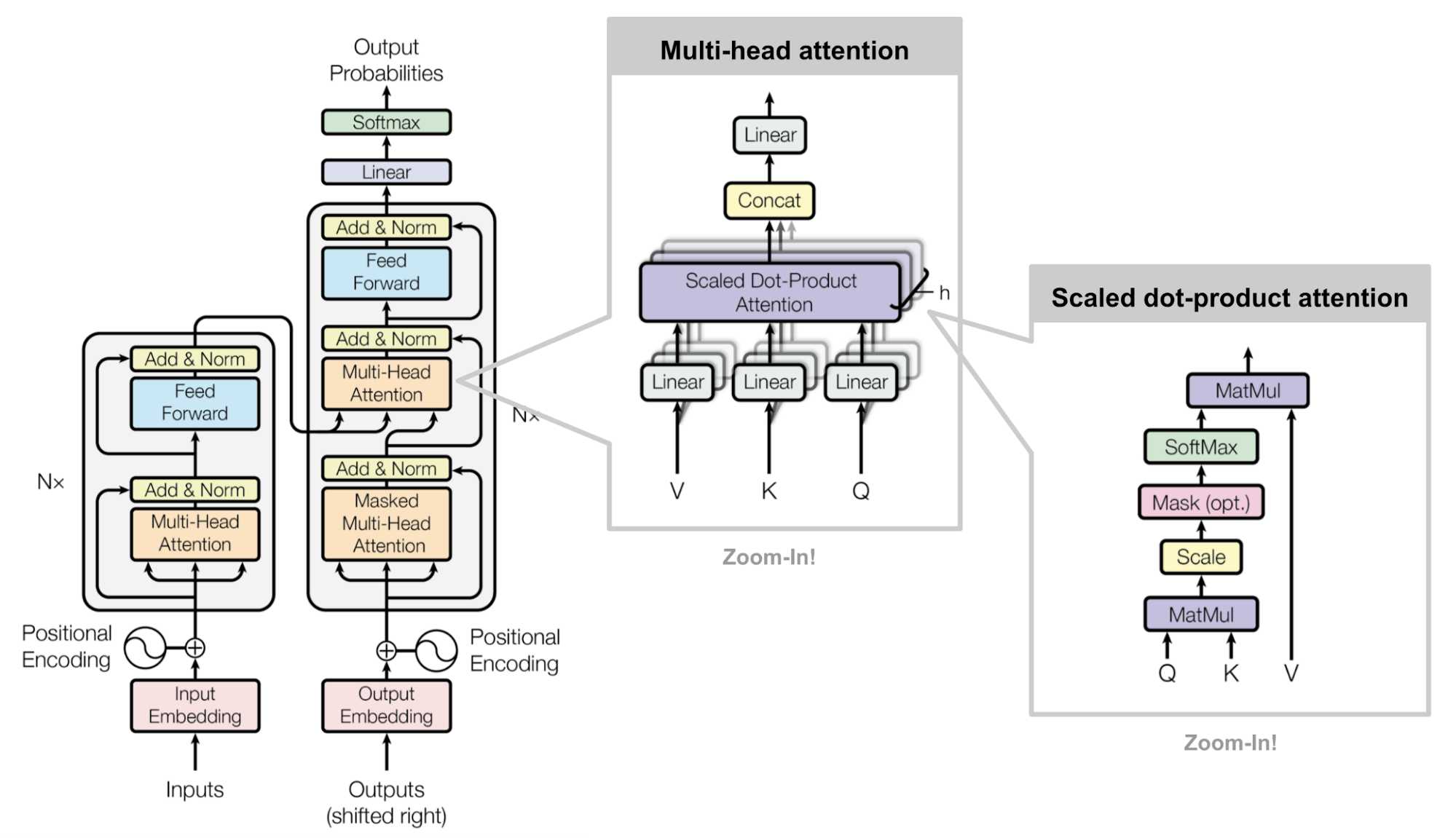Figure 4. The architecture of the vanilla Transformer. (Image source: Vaswani, et al., 2017)

Due to the great success of transformers, there are a lot of posts detailing the model architecture. I would recommend The Annotated Transformer by Alexander Rush which accompanies the original transformer paper by Vaswani, et al. with a PyTorch implementation. I will simply introduce with brevity the key mechanism of the transformer: multi-head self-attention.

We can understand the attention of the transformer as: with some input to attend to, taking in a query, with some attention method to produce an attention-weighted value of the input. For example, in the context of Seq2Seq NMT we introduced above, the input is the hidden states of the encoder, the query is embedding of last translated word, and the attention method we introduced is simple dot-product attention between the input and the query.

For the transformer, it understands the input as a key-value pair, $K, V \in \mathbb{R}^n$ , which is produced through some linear projections with learnable weights. The query is also projected as a vector $Q \in \mathbb{R}^n$ . The attention method is a scaled dot-product attention:

\text{Attention}(Q, K, V) = \text{softmax}(\frac{QK^T}{\sqrt{d}}V)

Multi-head attention runs through this scaled dot-product attention several times to produce different attention values. This is like we have several convolution layers to attend to different structural information.

References

[1] Sutskever, Ilya, et al. Sequence to Sequence Learning with Neural Networks. NIPS 2014.

[2] Bahdanau, Dzmitry, et al. Neural Machine Translation by Jointly Learning to Align and Translate. ICLR 2015.

[3] Ashish Vaswani, et al. “Attention is all you need.” NIPS 2017.